Introduction
We previously blogged about Detect Network beaconing via Intra-Request time delta patterns in Microsoft Sentinel using native KQL from This KQL query is complex in nature and often needs to operate on very large datasets such as network firewall logs in CommonSecurityLogs table. Even after applying optimization and baselining to reduce the original datasets, sometimes such complex operations do not scale well from Log Analytics especially when you want to analyze and compare large historical datasets with the current days data. In such cases you can offload expensive data manipulation and processing operations to services outside Microsoft Sentinel and bring actionable results back to continue hunting in Microsoft Sentinel.
In this first of 2-part blog, we will do notebook code and section walkthrough to show how you can leverage power of Apache Spark via Azure Synapse in Azure ML Notebooks to perform scalable hunting on large historical datasets to find potential network beaconing patterns. In second part, we will take a sample dataset and run the notebook on it to find potential beaconing traffic resulting from simulation of PowerShell Empire C2.
In general, the data pipeline and analysis architecture look like below.
Also special thanks to @Chi_Nguyen and Zhipeng Zhao for review , feedback on the blog and testing the notebook.
Apache Spark via Azure Synapse in Azure ML Notebooks
Pre-requisites
To use Apache Spark with Azure ML notebooks, you must first configure your data pipeline and connect Azure Synapse via linked service. You can check existing docs - Large-scale security analytics using Azure Sentinel notebooks and Azure Synapse integration for a step by step process and also use notebook Configurate Azure ML and Azure Synapse Analytics to set up Azure ML and Azure Synapse Analytics environment. Additionally, the notebook provides the steps to export your data from Log Analytics workspace to an Azure Data Lake Storage (ADLS) Gen2.
Loading the data
Once you have exported your logs to ADLS storage, you can connect to it and load the data required for analysis. In this case, we are going to load the current day’s dataset for analysis to find recent beaconing attempts. When you configure your data export to ADLS, it creates folder architecture per day, hour or granular 5-min buckets. Since the data is distributed across various folders, we need to programmatically generate the source path and load all the files underneath it.
Let’s start with specifying all the required parameters to generate ADLS paths. The ADLS storage file is combination of various attributes such as storage account name, container name, subscription id , resource group etc. We are also specifying additional input parameters such as device vendor, end date and lookback_days.
The below example cell shows where you can provide these details one time. Note: All the subsequent synapse cells start with %%synapse magic command. If you get an error on magic not found, run setup notebook and install required packages first.
Now once we have base path, data is stored across various directories.
Below example shows sample folder structure in the format year/month/day/hour/minute.
To generate such paths programmatically, we have created a function which accepts date and lookback period as input.
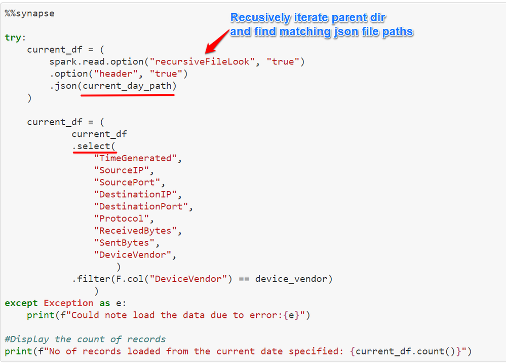
Finally, once we have generated current_day and historical_day paths, you can load the datasets as shown in below example cell. Here we have used below with additional options.
read : To read json file with additional options to keep the header and recursiveFileLook as true to recursively scan directory for matching files.
Note: recursiveFileLook is only available from Spark 3.1 so make sure to create Spark pool with 3.1 or above.
select: To select specified columns required for analysis.
filter: To filter by column value.
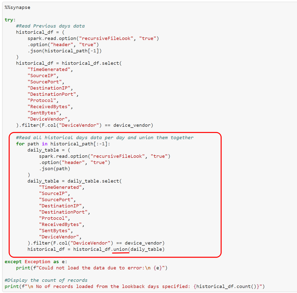
You can use a similar cell to load the historical dataset, where you can load individual files and union them together to load all historical data. Historical data will help in baselining the environment effectively, if you do not have historical data exported already, you can just run this on current data.
union: Union of individual days from historical days dataset.
Data Preparation
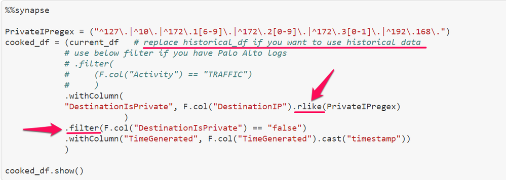
As we are looking for external network beaconing before we do the baselining, you can filter the input dataset to only IP address pair from Private to Public IP addresses. To do this, you can use regular expressions and the PySpark operator rlike. Once we have populated additional columns stating the type of destination IP, you can then filter only for public destination IP addresses.
In this cell, we have used below PySpark APIs
withcolumn : To create new column based on the condition.
rlike: To match with regular expression.
show: To show results after regex matching and filtering.
Scalable Baselining across Historical Data
If you have historical dataset (lookback days from 7 to 30 depending upon the availability) loaded , you can perform baselining on it. Baselining can help reduce false positives by removing frequently occurring public destinations which are likely benign. You can take various baselining approaches to reduce input dataset.
In this notebook, we are going to use few static thresholds. You can also use dynamic logic in terms of percentages across total hosts in your environments if the thresholds are too low or high.
- daily_event_count_threshold : minimum number of events in a day. Default value set to 100. Any source IP addresses below threshold will be ignored.
- degree_of_srcip_threshold: max number of sources IP addresses per destination IP. Default value set to 25. Any destination IP addresses above this threshold will be ignored.
Once we identified both source IP and destination IPs from the baselining, you can further join this with the original current dataset to find beaconing patterns.
Below cell shows such baselining operations along with spark APIs.
groupBy : Groups dataframe using specified columns so we can run aggregations on them.
orderBy: Returns new dataframe sorted by specified column.
agg: Aggregate entire dataframe.
countDistinct: Return distinct count of column.
alias: Returns column aliased with new name.
join: Join another dataframe such as csl_srcip, csl_dstip.
Data Wrangling using Apache Spark
Once we have finished loading current data, historical data , prepare the dataset by filtering via regex and apply baselining to it, we can perform additional transformations on the PySpark dataframe.
- Sort the dataset by SourceIP.
- Calculate the time difference between first event and next event.
- Partition dataset per Source IP, Destination IP or Destination Port
- Group dataset into consecutive 3 rows to calculate the Timedeltalistcount which is aggregate of 3 respective timedelta counts
- Calculate percentagebeacon between TotalEventscount and Timedeltalistcount
- Apply thresholds to further reduce false positives
Windowing
In the first step, we have sorted dataset and partitioned per SourceIP to calculate the time difference between the first and next row.
Window: Utility function for defining window in dataframe. In this case, we have created windows by partitioning by SourceIp first and later by multiple fields; DeviceVendor, SourceIP, DestinationIP, DestinationPort.
Time Delta Calculation
In this step, we have used lag to calculate time delta on the serialized and partitioned data obtained from previous step.
lag : Returns value that is offset rows before current row. In this case, we are calculating time delta between two consecutive events.
unix_timestamp: convert time string to Unix time stamp (in seconds) to return timedelta in seconds.
We have also performed multiple aggregations to populate additional columns as shown in the screenshot.
sum : Computes sum for each numeric columns for each group.
count: Returns number of rows in dataframe.
Repartition and Calculate Percentage Beaconing
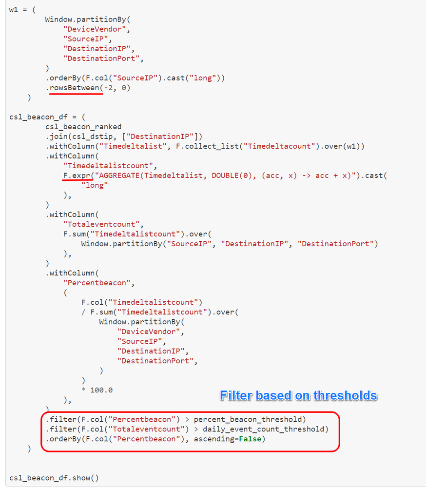
Now, we can create a window specification with frame boundaries of 3 rows by partitioning based on DeviceVendor, SourceIP, DestinationIP, DestinationPort and order it by SourceIP in . This step will group dataset into consecutive 3 rows to calculate the Timedeltalistcount which is an aggregate of 3 respective timedelta counts.
Rowsbetween : Crates window spec with frame boundaries defined from start (inclusive) to end (inclusive).
Expr : Parses expression string into column. In this case we are calculating sum values of array integer.
Aggregate : aggregate(expre, start, merge,finish) – applies binary operator to an initial state and all elements of array and reduces this to a single state. In this case, we are aggregating all the timedeltalist and calculating respective sum of each.
We have also calculated PercentageBeacon which will be =
Aggregated count per time delta or list of time delta/ Total Events for Source-DestinationIP-Port * 100.
Export Results from ADLS
Now you can export potential beaconing results retrieved from previous step and export it locally to be used outside the Azure Synapse session. To do, we have used SPARK API coalesce.
Coalesce: You can specify number of partitions (e.g. 1) to output dataframe results into single json file and write back to ADLS in the specified directory.
You can then stop the session by executing %synapse stop.
Once you are outside of synapse session, you can then download the output from ADLS locally and perform various data analysis, enrichment operations.
Specify the input parameters for ADLS account again since it is outside synapse session, it won’t recognize the variables declared inside synapse session.
Enriching entities with MSTICPy for investigation
In order to investigate the beaconing results , we can further automate the entity enrichment tasks such as GeoIP lookup, Whois lookup and ThreatIntel lookups using native features of MSTICPy library.
You can also visualize results onto geographical map using FoliumMap visualization of MSTICPy.
Please refer MSTICPy data enrichment and visualization for detailed information along with example notebooks. Once you have enriched results, you can then send those results back to Sentinel as bookmark by using MSTICPy Microsoft Sentinel APIs.
Conclusion
The notebook implemented use case outlined previously in the blog using Apache spark , applied baselining methods on historical datasets to further reduce datasets and also enriched entities with useful information using MSTICPy features to automate common investigation steps for analysts. You can further take these results into Microsoft Sentinel to either combine with other datasets or alerts to increase fidelity or create incidents to investigate the reasoning behind the patterns observed. In the second part of the blog, we will take simulated datasets to test this notebook and analyze the results.
References
- Detect Network beaconing via Intra-Request time delta patterns in Microsoft Sentinel - Microsoft Tech Community
- Guided Hunting Notebook : https://aka.ms/Beacon_Synapse_Notebook
- Apache PySpark SQL : https://spark.apache.org/docs/3.1.1/api/python/reference/pyspark.sql.html
- Introducing Window Functions in Spark SQL - The Databricks Blog
- https://stackoverflow.com/questions/47839077/pyspark-best-way-to-sum-values-in-column-of-type-arrayinteger
- https://msticpy.readthedocs.io/en/latest/data_acquisition/GeoIPLookups.html
- https://msticpy.readthedocs.io/en/latest/data_acquisition/TIProviders.html
- https://msticpy.readthedocs.io/en/latest/visualization/FoliumMap.html


